College Football - The Great Flattening

Some of us saw this coming decades ago.

College football fans may finally be witnessing the achievement of a long sought white whale—the ever elusive “parity”. Claims of its arrival have been echoing for decades. But every rumor of life for this goal was greatly exaggerated.

The reason it remained so elusive is that the NCAA has always been a cartel dominated by the large programs who exerted their power to their advantage. The sports economics literature goes back famously on this to Fleisher, Goff, and Tollison, but it predates that by decades. My contribution is here.

With the recent changes stemming from the supreme court rulings in NCAA v. Alston (2021) and O’Bannon v. NCAA (2015) but also dating to NCAA v. Board of Regents of the University of Oklahoma (1984), we are now truly seeing a leveling of the playing field. As I’ve warned before, parity won’t look like many imagine it. You cannot achieve momentous change without, well, momentous change. More precisely, you cannot just bring about one very different outcome without inviting a vast host of other differences in structure and outcome.

The development of changes to transfer rules and the transfer portal itself, the recognition of property rights in name, image, and likeness (NIL), and the evolution of league structure (conference realignment, an effect as much as cause here) have created a new paradigm for college football. To be sure these are works in progress. It’s not done, but there is no going back. More changes like perhaps a super league (upper division of FBS) could well be on the horizon.

The Claim

How do I make the claim that we are now seeing something like a movement to greater competitiveness in college football, which is a much better, more precise claim than “parity”¹? Simply by looking at the dispersion of talent among the top 50 ranked teams in recruiting of high school players.

Recruiting rankings have shown a flattening effect whereby the difference between the highest ranked teams in a given year and the bottom of the top 50 is significantly smaller recently than it was over the past 25 years. In plain English the concentration of talent is less today than it has been.

Before we get to the evidence, it is important to note that this still might not mean greater competitiveness—proof would be in the outcome rather than the inputs. A great start would be too look at the Noll-Scully measure of competitiveness. In a nutshell this is a comparison of how much Win-Loss dispersion there is between teams in a given year throughout a league compared to what we would expect by chance IF teams were perfectly matched in all cases (i.e., every game was a 50-50 tossup). Although this metric has its weaknesses, it is a fairly robust way to test for changes in competitiveness.²

There are several hypotheses worth considering to challenge the idea I’m putting forward that less unequal distribution of player talent will have the effect of leveling the playing field. For one, perhaps players don’t matter that much. This seems highly unlikely intuitively, and a cursory look at the evidence might allow us to reject this without further examination. The top named teams in recruiting are very consistently the top teams in Win-Loss record. There is a reason for the old adage “It ain’t the Xs and the Os, but the Jimmys and the Joes”.

Another hypothesis is the traditional dominant teams might be allowing players to go to lower programs with the idea they would farm them back into their own once proven (or leave them where they first land when they don’t pan out).

This requires quite a bit of foresight and implies quite a reach to be true. It might still allow for more competitiveness just with more player turnover into and out of programs big and small. In fact it evokes the failed idea of predatory pricing presuming the incumbent interests can exert an undue influence. Every attempt to find this theoretical market failure fails upon examination—firms of old like Standard Oil and of new like Walmart and Amazon don’t drive out small competitors and then raise prices enjoying market power. They simply foster a more competitive environment for the benefit of consumers. Similarly I doubt this farm-team strategy is a strategy at all much less a workable one. The biggest programs are subject to these new competitive forces rather than the beneficiaries or drivers of them.

The new competitive landscape of college football has the big programs still competing against each other for talent, and now they are also competing against smaller programs. Talent is spreading far and wide followed by annual reshuffling. Not only can lesser programs recruit better against the top programs for high school players, they can also poach them too. No, I’m not saying the non-traditional powers like Kansas are going to start taking starters from Oklahoma. But they can take Oklahoma’s backups. My expectation is that the transfer portal today with the help of now legal (above-the-table) payments to players will likely flatten the difference between teams even more. There is a reason the biggest complaints about the new world of college football come from the top programs. Their oligopoly power they dominated with, from the under-the-table arrangements to limiting the dimensions of competition explicitly, is threatened like never before.

An analysis of that secondary market effect remains for another day (and post). For now let’s focus on the primary market of high school player recruiting.

The Evidence - Total Points Gap

Using the team recruiting rankings from 247sports.com, I compiled the final rankings for all the years since their dataset begins in 2002. I also have the years 2000 and 2001, but these are incomplete so they are excluded from the analysis below.

You can download my workbook and check me for replicability as well as errors here. I’m not sure if the graphs come through. If you’d like an Excel version, please contact me. I would be happy to share the .xlsm file.

The analysis below shows that over the years the difference between the top teams in the rankings and the teams at the bottom of the top 50 has lessened considerably.

247 scores each team’s recruiting class giving it a point value. For 2026 the #1 class is USC with a score of 305.47 while the #50 class is Kansas State with 203.62—a gap of 101.85. In 2015, to pick a random year, the gap between #1 Alabama and #50 Virginia was 131.18. Anecdotally, this shows more competitiveness in 2026 than in 2015. The same is true when looking at 2002 where the gap was 163.72 between #1 Texas and #50 West Virginia. (See the postscript at the bottom for the inspiration of looking deeper at this).

I wanted to know if a more thorough analysis would prove this anecdote to be supported. It did.

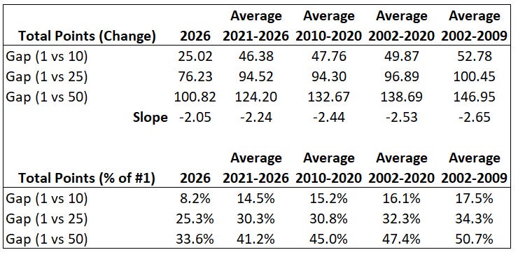
Here is a graphical look at the rankings for 2026 and the average for groups of years. Notice that the lines are flattening significantly.

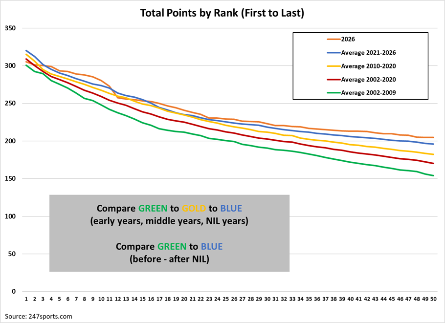
All the gain is at the bottom with actually some improvement at the top. This might indicate that the gains to the bottom teams are coming from better acquisitions at the expense of teams further down the rankings. See the note at the bottom about expanding the analysis as well as the caveats. Another thing to consider is if the data is consistent throughout the period examined (2002-2026). I believe it is based on my understanding of 247’s recruiting methodology, but this remains an area to examine.

Another way to look at it graphically is to look at every year. Admittedly this is noisy, but my use of color changes hopefully allow you to see the differences.

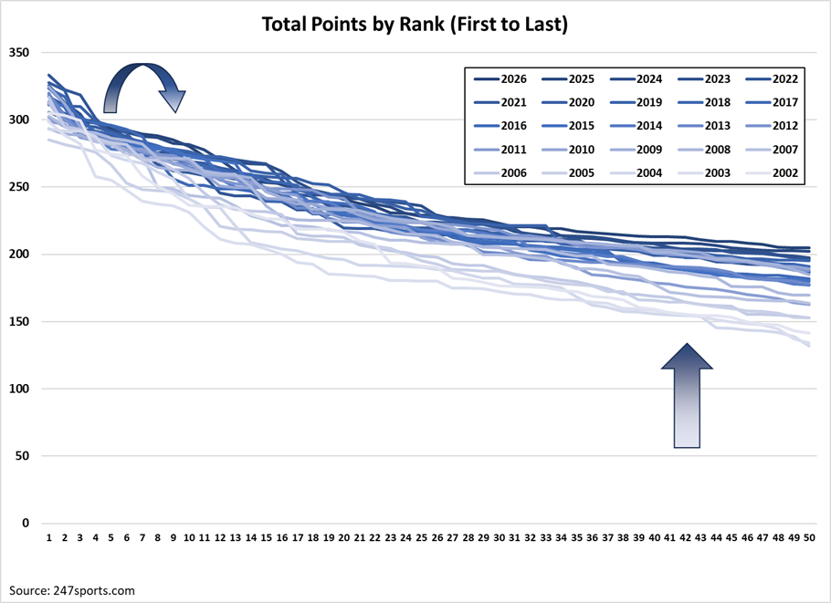
As I will note below in the persistence section, it seems the scores for the top recruiting teams bottomed in the middle of the dataset. Hence, my use of the rotating arrow.

My major contention from this is that the gap is narrowing (lines are flattening) meaningfully. In fact there are 30-50% reductions in the total point gaps (see the tables below for details). This represents a lot more competitiveness in recruiting. The top teams are still getting the top players, but now the teams well below the elite level are doing so too.

The Evidence - Points per Commit

It could be argued that especially in this latest era of college football teams seek to gain recruits where they are needed most. This can mean that teams don’t recruit as many players out of high school signing them as recruits as they did in the past. Or perhaps they try to absorb as much talent as they can signing a very large class. This would have the effect of changing the total points simply by virtue of there being more or fewer recruits.

To wit in 2026 some teams had as many as 49 commits signed while others in the top 50 had as few as 14. This is not a new development as this type of variance is seen throughout the dataset.

The transfer portal as well as changes to the signing rules could be distorting total points. It is for this reason that I wanted to look at the full curve rather than just he gap between #1 and #50. Still, we should consider the points per recruit (commit) to control for this.

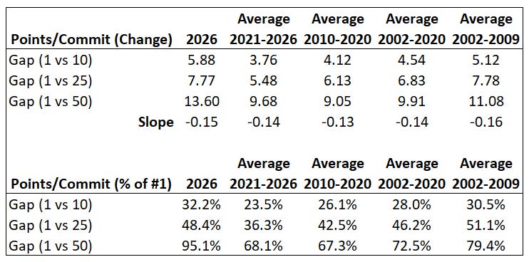
To make the adjustment I simply reranked all top 50 every year on the points/commit metric (total points divided by number of recruits signed). Here are the results.

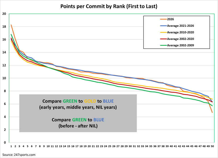
Again we see the same indications of much more competitiveness in the most recent era. In fact the curves rise significantly in the middle and stay higher down to the #50 team. It appears 2026 might be aberrational since it stands out as compared to the 2021-2026 grouping for which it is a part.

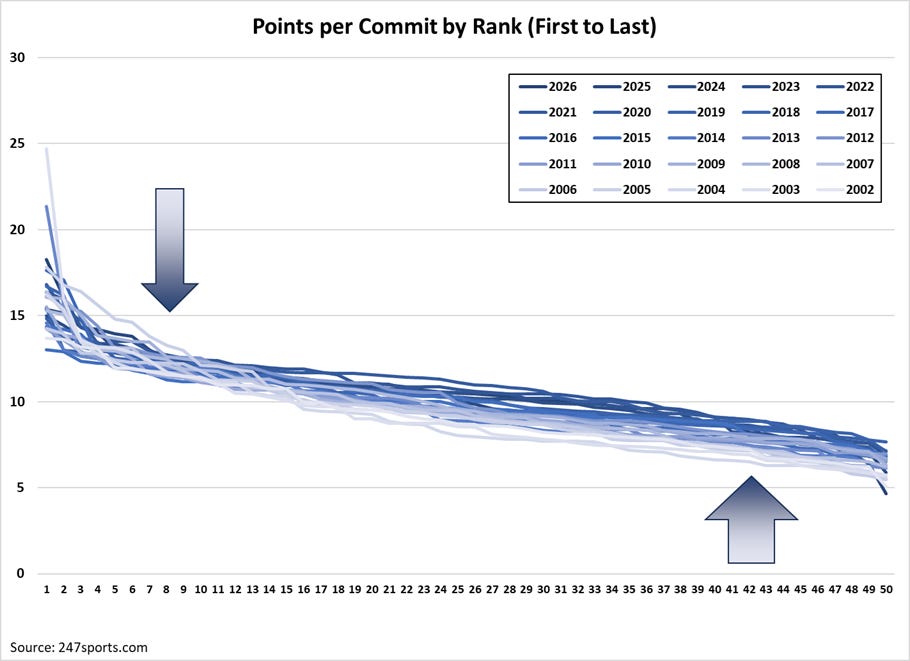
We see the same when looking at year by year comparisons.

To summarize this evidence I present the tables for the data and analysis. My apologies for its width (small font). Hopefully clicking on it will make it bigger.

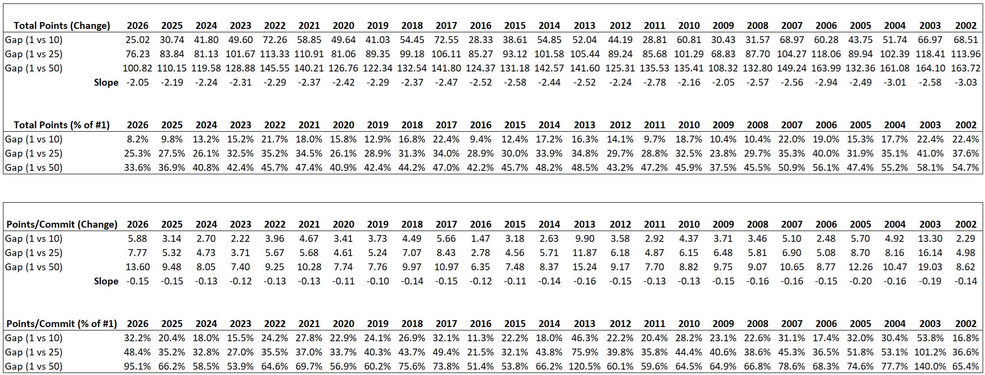
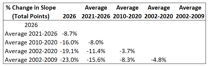
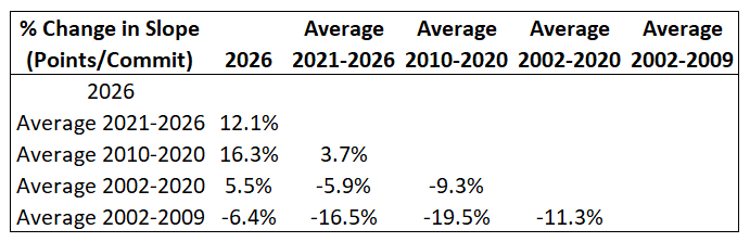
As I observe above and below, there does seem to have been some flattening prior to the latest era—compare 2002-2009 to 2010-2020. Perhaps the NIL-transfer portal era simply is not the only factor at play. Regardless, the acceleration of this trend as well as the apparent emergence of a new, meaningful phase of it must be considered.

The points/commit metric does not show as substantial a reduction (or any at all in some cases) in slope—the flattening is less apparent or nonexistent. So perhaps the top teams are better at getting the best talent per recruit? Not so fast, as the teams at the top of the rankings in points/commit are not the same teams at all. This metric has its own limitation (noise) to consider. In fact the top teams in this reranking tend to be the teams with fewer recruits—oftentimes below replacement level as they are below 20 (teams can only have 85 scholarship players on the roster in a given year with four years plus redshirt for typical eligibility). You’ll have to download the entire workbook to see this for further examination. Suffice it to say there is not a perfect metric here.

A Note on Persistence

One way to examine the flattening is to look for persistence—how much year-over-year turnover is there in the list. For this I looked at the number of new teams from the prior year, from a year 10 years prior (for each year 2026-2013), and comparing each year versus 2002.

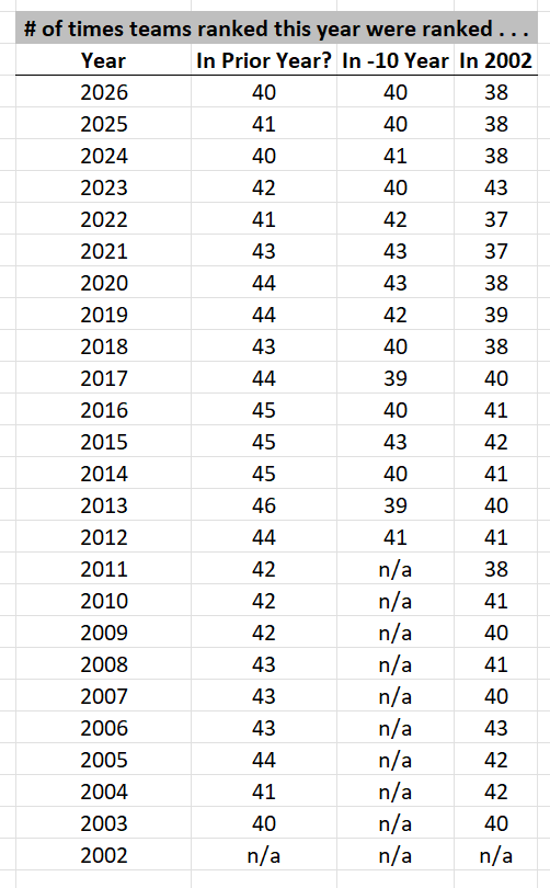
Looking at this shows A LOT of persistence. New teams aren’t entering the fray (rankings). And they never have. Out of 50 teams ranked, very consistently there are about 10 new teams in the rankings in all three comparisons. So we aren’t seeing the volatility many might suppose (hope?) would occur. At least not yet.

I also looked at the number of times teams ranked for the years 2021-2026, 2015-2020, and 2009-2014 were ranked in the prior 6 years, prior 6 years 6 years back, and prior 6 years 12 years back. I was looking to see how many times there were, for example, 6 teams ranked in both 2021-2026 as well as the prior 6 years (2015-2020), prior 6 skipping back 6 years (2009-2014), and prior 6 skipping back 12 years (2002-2008). I did this looking for 6, 5, 4, 3, 2, 1, and 0 teams repeating. The idea is there is evidence for more turnover if fewer teams are in the rankings both now and in the prior periods. The most you can have is 6 since that would mean a team was in the rankings every year in both periods examined.

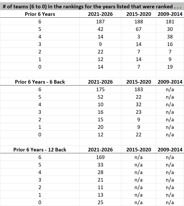
Reading the results in the first grid shows that 187 times 6 teams in the 2021-2026 were in the rankings each year of 2021-2026 and in the rankings 2015-2020. Basically no change from the cohort 2015-2020 (looking back to 2009-2014 for them). But there were 14 teams in the 2021-2026 rankings that were not at all in the 2015-2020 rankings while it was only 7 teams in 2015-2020 that were “new” compared to 2009-2014.

The result is stronger in the 6 years 6 years back second grid for teams repeating all six years as well as some others (6, 4, and 3 all show this). Yet the number of newcomer teams (the 0 line) shows fewer newcomers (12) in the 2021-2026 versus 2015-2020 (22). The third grid is more informational as it doesn’t have a comparable group. However, it does show the general case of turnover itself comparing it vertically to the first two grids.

So, this is a mixed result, but it does have some indication that there is more turnover especially when comparing the teams in the six-year period 2021-2026 against the cohort 2015-2020. This also shows up comparing 2021-2026 vertically for prior 6 versus prior 6 years 6 years back but reverses versus prior 6 years 12 years back. This will again come into play in the next analysis as it looks like turnover bottomed out in the middle of the dataset.

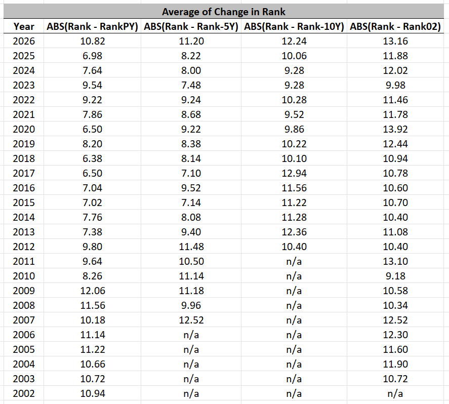
Additionally I looked at the change in team rank. To do so I considered both the variance in change of rank and the average change in rank looking in both cases for each year to the prior year, 5 years back, 10 years back, and since 2002 periods. In both cases the story is mixed as for the most part turnover in where teams are ranked bottomed out (became the least competitive) in the middle of the dataset (~2015 through ~2020) with the recent period being a movement back to the highest levels of turnover (more competitive today than in the middle of the last 20 years).

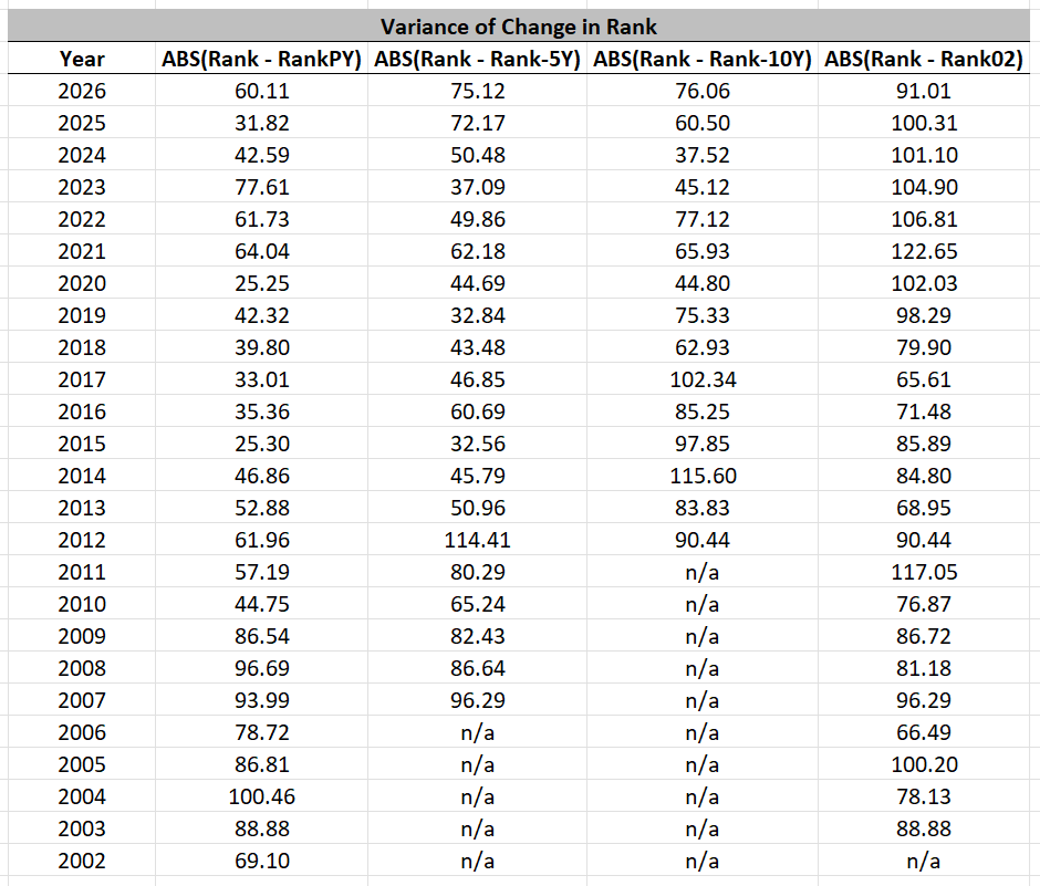
It seems that persistence has been through a cycle from lower to higher and now back to lower. I am interested in other ways to dig into this as it certainly has implications for competitiveness in recruiting. And it should bear out eventually in competitiveness on the field.

Conclusion

The evidence as presented seems to strongly indicate that competitiveness in college football recruiting is rising. More teams are doing better in recruiting than in the past looking over the recent 25-year span.

P.S. This analysis could be taken further by expanding the dataset beyond the top 50 teams. 247’s rankings go as deep as ranking the 202nd team in 2026. But perhaps it would need to be capped at the top 100 since as recently as 2015 the rankings only extend to 125th and 110th for 2002. There would be another potential problem as the data expanded for more ranks as the integrity might suffer. Additionally, there would be very few data points for the scoring at the lowest ranks potentially introducing base effects.

P.P.S. HT to this X.com post by Bud Elliot which is what brought this to my attention and inspired the deep dive.

1. I have long contended that this is a bad word to employ since it literally means equality, something that is both impossible to achieve in a reasonable sports domain as well as being undesirable. The interest in a league that had every contest in every season be a 50/50 game of chance would be orders of magnitude smaller than what is seen in sports as we know it.

2. It is important to note that it is problematic to compare competitiveness between leagues (e.g., NFL vs. CFB, NFL vs. MLB, etc.) as the difference in season length distorts the ratio. For college football, this would only be a small problem since teams have been playing a 12-game regular season since 2006 (2020 notwithstanding) and played 11 games before that. As I understand it, the major problem with Noll-Scully really comes about with major changes in length like baseball versus football. At least that is what Gerald Scully told me when I spoke with him years ago as part of my formal research.